


1. Introduction
How do parties translate public preferences into policy in multiparty systems? The link between public preferences and government actions lies at the heart of democratic governance, leading generations of scholars to investigate questions of policy representation and responsiveness. A large majority of this research, however, focuses on countries characterized by single-party governments, such as the United States, the United Kingdom and Canada.Footnote 1, Footnote 2 In coalition governments, public opinion also influences parties’ policy preferences but the implementation of any coalition member's preferences into actual policy requires an extra step: coalition bargaining.
Until now, no strategically oriented, dynamic and empirically validated means of predicting which party's preferences will emerge as policy has existed. Some scholars, of course, have nonetheless analyzed the influence of public preferences and policy outputs in multiparty systems (e.g., Klemmensen and Hobolt, Reference Klemmensen and Hobolt2005; Wlezien and Soroka, Reference Wlezien and Soroka2012) but they have done so by neglecting the policy bargaining stage. Scholars wishing to acknowledge that parties’ policy preferences do not translate directly into policy outputs in multiparty governments had only two choices: they could (1) turn to static measures such as seat allocation rules (e.g., Gamson, Reference Gamson1961) and/or bargaining power indices (Shapley and Shubik, Reference Shapley and Shubik1954; Banzhaf, Reference Banzhaf1964) or (2) posit that parties’ standing in the polls or shifts in public opinion on specific issues over time alter the balance of power in coalition governments (e.g., Lupia and Strøm, Reference Lupia and Strøm1995).
We draw on key insights from both of these approaches to develop a novel measure of bargaining leverage in coalition governments. Like Shapley and Shubik (Reference Shapley and Shubik1954), we argue that bargaining leverage arises from credible threats to quit the government and, like Lupia and Strøm (Reference Lupia and Strøm1995), we argue that the credibility of such threats varies dynamically over the life of a government as external circumstances and polls change. We differ, however, by arguing (and demonstrating) that most shifts in party polling and public opinion are not sufficient to change bargaining outcomes and, hence, policy. Shifts in polling only change bargaining leverage and policy outcomes when they also change a party's ability to participate in an alternative government. Thus, what matters in dynamic negotiations over policy in coalitions is how changes in external polls affect parties’ probabilities of inclusion in alternative governments: coalition inclusion probabilities.
We also differ from these theoretical literatures in our empirical focus. We build an empirical coalition formation model that we optimize for prediction with out-of-sample testing and then apply to a large sample of polls. We can thus predict the probability of every possible coalition that could form at each point in time and then sum by party to calculate the probability of each party entering government. Numerous variants of coalition inclusion probabilities (CIPs) are possible, depending on the application and whether one wishes to calculate, say, a given party's leverage vis-à-vis a specific bargaining partner by calculating the probability of the first party entering a government that excludes the second. The project described in this paper calculates a set of CIPs for most parties in 21 parliamentary democracies at a monthly frequency for all periods in which data exist between 1970 and 2018.
Consequently, we make publicly available a set of measures that, in combination with other variables, should enable scholars to better predict party behavior and policy outcomes in multiparty governments. We demonstrate our measures’ utility with two distinctly different applications—government spending and the stringency of environmental policies—and contrast the performance of CIPs with weak results from naïve alternatives that neglect coalition bargaining: political polls, seat shares and public opinion.
2. How to predict policy
2.1 Public opinion
Scholars have made large strides explaining and predicting policy in settings with single-party governments. Research on the United States, United Kingdom and Canada has shown that public preferences on issues generally cluster across issues, suggesting a single underlying preference for government action (Stimson et al., Reference Stimson, MacKuen and Erikson1995) but also that some salient issues can deviate and influence policy (Druckman and Jacobs, Reference Druckman and Jacobs2006), that policy mood responds to the economy (Durr, Reference Durr1993), that policy change often precedes changes in public opinion (Page and Shapiro, Reference Page and Shapiro1983), that governments shift policy dynamically in response to public opinion between elections (Stimson et al., Reference Stimson, MacKuen and Erikson1995), and that policy and public opinion interact “thermostatically” with each influencing the other (Wlezien, Reference Wlezien1995; Soroka and Wlezien, Reference Soroka and Wlezien2010).
Research that addresses multi-party systems, however, has yielded notably fewer and less precise findings predicting policy outcomes. We do know how broad policy outcomes differ in systems with single-party and multi-party governance—policy responsiveness is slower (Wlezien and Soroka, Reference Wlezien and Soroka2012) in many of the countries in which policy changes come in infrequent but large clusters (Baumgartner et al., Reference Baumgartner, Breunig, Green-Pedersen, Jones, Mortensen, Nuytemans and Walgrave2009)—but more fine-grained questions about which party successfully implements its preferred policy and in what circumstances elude us.
So, why does policy research do so much better in single-party government settings? The reason, we argue, is that predicting policy from coalition governments requires understanding the bargaining leverage of the parties, a step that is not necessary with single-party majority governments. Interestingly, one important and highly visible finding that does address policy outcomes in multiparty systems posits coalition negotiations and compromise as the reason why policy outcomes in coalition governments hew closer to the public opinion preferences of the median voter in proportional than in majoritarian electoral systems (Huber and Powell, Reference Huber and Powell1994; Powell, Reference Powell2009). What they do not address, however, is how coalition members reach a compromise. It is precisely this process and how it influences policy in favor of which actors that we seek to address here theoretically but, most importantly, through the creation of a new tool.
2.2 Elections and polls
Electoral competitiveness, like public opinion, also serves frequently as a predictor of policy. In contrast to public opinion that usually concerns a particular issue, however, electoral competitiveness is most often associated with how well, closely or quickly governments respond to a valence issue or shift policy toward the preferences of the greatest number of voters. Politicians elected in competitive settings, for example, purportedly respond more to their median constituents (Ansolabehere et al., Reference Ansolabehere, Snyder and Stewart2001), moderate their partisan preferences in fiscal policy (Solé-Ollé, Reference Solé-Ollé2006) and spend more on public goods (Hecock, Reference Hecock2006).
Measuring electoral competitiveness, however, is not so straight-forward. The strong over-representation of single-country studies in research related to electoral competitiveness, most notably the United States and other countries with frequent single-party government, is likely a result of the ease of measuring competitiveness with two-party vote-, poll- or seat-margins in such systems.Footnote 3 The dependence of such margins on the number of parties in the system makes it an awkward measure for cross-national samples that include multiparty systems. Given that a minority of developed democracies host two-party systems, cross-national research requires a measure of electoral competitiveness that also captures patterns of party competition in multi-party systems.
Recently, a few cross-national measures have emerged, each presenting a distinct way of conceptualizing and measuring multi-party electoral competitiveness as electoral vulnerability (Abou-Chadi and Immergut, Reference Abou-Chadi and Immergut2014), the probability of the party with the most seats in parliament losing its plurality (Kayser and Lindstädt, Reference Kayser and Lindstädt2015), bargaining power categories (Abou-Chadi and Orlowski, Reference Abou-Chadi and Orlowski2016) and electoral availability (Wagner, Reference Wagner2017). Electoral competitiveness may indeed influence parties’ policy positions but predicting party positions is not the same thing as predicting policy. Regardless of how well electoral competitiveness predicts parties’ policy positions, even in multiparty systems (see, e.g., Adams, Reference Adams2012), it does not and cannot address the fact that policy outcomes in most coalition governments are the outcome of coalition bargaining rather than the preferences of any single party. In other words, an intervening and crucial step—coalition bargaining—exists between electoral competitiveness (usually based on vote, seat or polling outcomes) and policy in multiparty systems with coalition governments.
Nor can one simply assume that increases in vote, seat or poll shares will map monotonically onto the probability of a party advancing its preferred policy. For example, one strong factor influencing policy is inclusion in government but simply increasing vote and seat share will not necessarily increase a party's chance of gaining office. A party that shifts from the third to the second largest seat share in a parliament, for example, might actually reduce its probability of government inclusion because the largest party might, following Gamson's law, prefer the third largest party as a coalition partner in order to dole out fewer portfolios. What matters for predicting policy and parties’ behavior, we argue, is often not polls, vote shares, seat shares, measures of electoral competitiveness or even public opinion but the specific set of coalition formation options and bargaining leverage that parties hold.
2.3 Bargaining power and policy positioning
In coalition governments, bargaining between coalition members determines policy while future coalition opportunities partly determine parties’ preferred party positions. Thus, both current coalition conditions (via bargaining leverage) and future coalition prospects (via strategic policy positioning) influence policy.
2.3.1 Bargaining leverage
When multiple parties with differing policy preferences are in government, bargaining leverage matters for policy-making. When a party can credibly threaten to abandon the government for an alternative governing coalition, especially one that excludes the leading party, it has considerable influence. This assertion is not novel. Over half a century ago, the authors of several voting power indices generated algorithms to calculate the power (weight) of each vote (party) as a function of its probability of causing a coalition to form or fail by switching (Penrose, Reference Penrose1946; Shapley and Shubik, Reference Shapley and Shubik1954; Banzhaf, Reference Banzhaf1964). Exit threat is the key idea of voting power indices (e.g., Banzhaf, Reference Banzhaf1964) and outside options are key to coalition members’ leverage (Becher and Christiansen, Reference Becher and Christiansen2015). Voting power indices and work on bargaining weights remained mostly theoretical, however, because they omitted key constructs such as party ideology that empirically matter for coalition formation.
But can parties credibly bargain over policy in the first place? The outcome of bargaining in early models of coalition formation was primarily portfolio allocation rather than policies. An early and seminal model of coalition formation posits that informational and agenda setting advantages turn ministers into “policy dictators” in the portfolio of their ministries (Austen-Smith and Banks, Reference Austen-Smith and Banks1990; Laver and Shepsle, Reference Laver and Shepsle1996). Thus, credible policy compromise between parties is not possible, only compromise about which party controls which ministry. Policy-making in these approaches boils down to a collection of the ideal points of the parties holding given portfolios.
Later research, however, highlights the role of institutions in policing the coalition bargain (for a review, see Martin and Vanberg, Reference Martin, Vanberg, Gandhi and Ruiz-Rufino2015). Parties, in this approach—most recently articulated by Martin and Vanberg (Reference Martin and Vanberg2020) in the framework of bargaining along a contract curve—are able to reach policy compromises in which parties holding a portfolio agree to a policy position deviating from their ideal point. Policing by junior ministers (e.g., Thies, Reference Thies2001), legislative review (Kim and Loewenberg, Reference Kim and Loewenberg2005; Martin and Vanberg, Reference Martin and Vanberg2011) and coalition agreements (Klüver and Bäck, Reference Klüver and Bäck2019) can ensure that legislative drafts coming from ministries adhere to the bargain despite the temptation of “ministerial drift.”
2.3.2 Dynamic bargaining and strategic positioning
Policy compromises, regardless of how they are codified and enforced, are not set in stone. Policy outcomes can differ considerably from what was originally agreed following an election, for example, for the simple reason that circumstances change. Lupia and Strøm (Reference Lupia and Strøm1995, e.g., p. 649), on whose argument we build, posit that bargaining in coalitions over the life of a government is influenced by changes in parties’ standings in the polls: “The anticipation of good electoral fortunes gives a party a bargaining chip that it can exploit by either negotiating the balance of power within an existing coalition, forging a more attractive coalition with new partners, forcing dissolution and new elections, or protecting the existing cabinet.” What we add, however, is the contention that parties’ leverage does not rely on anticipated electoral performance (polls) but, more specifically, on how such an electoral performance would translate into coalition options. Such changes in coalition leverage can then be converted into policy changes without, as Martin and Vanberg (Reference Martin and Vanberg2020) note, the formal rebalancing of power in a coalition.
We adhere to this understanding of coalition formation, bargaining leverage and cross-portfolio policy compromise. We also extend it in two ways that speak to the primary theoretical contribution of this paper, the argument that parties’ CIPs predict policy. First, we posit that bargaining leverage in the form of coalition inclusion probabilities (exit threat) but also calculations about parties’ policy positions for their future coalition options (strategic positioning) affect policy outcomes. A party may benefit from adopting a policy position in a portfolio that it holds that deviates from its ideal point if that position is likely to offer it more or better coalition options whenever the next government is formed. Second, while previous research has investigated how parties form coalitions and coalition agreements, we introduce a dynamic understanding of parties over the life of a coalition that seeks to explain when parties, in response to polling information and forward-looking coalition calculations, break coalition agreements by demanding a new or revised policy.
2.4 Why CIPs matter
So, why do we need coalition probabilities to measure bargaining leverage? Why not capture leverage by employing expected seat shares which, in PR systems, map closely to expected vote shares and polls, to capture leverage? We have already noted that vote and seat shares are poor predictors of policy because they neglect policy bargaining in coalition governments, but could they themselves not serve as a measure of bargaining leverage? One might expect a party to have stronger outside options and, hence, a more credible exit threat if its polling numbers are strong. Political polling, in addition, is conducted regularly over the term of governments in most developed democracies, so could offer a dynamic measure of parties’ strength. Seat shares, of course, map closely to vote shares in PR systems.
Our answer, in short, is that inclusion in government plays a critical role in most parties’ objective functions and seat shares do not map smoothly onto the probability of parties being included in government. We illustrate this point with a simplified theoretical example that shows the relationship between seat shares and coalition inclusion. Figure 1 plots the probability of each of three parties being included in government as a function of the seat share of the first party (Party A).Footnote 4 Two observations from the figure are critical to our argument that coalition inclusion probabilities, not expected seat shares, should matter for bargaining leverage if parties seek participation in government. First, coalition inclusion probability is not a continuous function of seat share and is not necessarily monotonically related to seat share. Second, a party's vote share (and, hence seat share) can vary considerably within certain ranges without changing its coalition prospects at all. At given points, however, CIP jumps up (or down) to a new value. Seat shares, therefore, are a poor guide to predicting parties’ behavior even if expected seat share is conceived of as a measure of bargaining leverage. The results that we show later in this article that CIPs, but not seat shares, predict policy can thus be interpreted as evidence that parties care more about inclusion in government than seat shares, per se.

Fig. 1. Theory—CIP versus vote shares. Coalition probabilities plotted against Party A's seat share. Note that CIPs are not a continuous function and are not necessarily monotonic.
2.4.1 An illustration: the German government of 2009–2013
The influence of coalition inclusion prospects on party behavior is not only a theoretical matter. Before addressing empirical estimation in the following section, we illustrate here how changing coalition calculations can influence party position taking and governmental policy outcomes via both exit threat and strategic positioning with an example from one government in Germany.
After their victory in the 2009 election, the German Christian Democratic Party (CDU) and their Bavarian sister party, the Christian Social Union (CSU), chose to form a government with the resurgent Free Democratic Party (FDP), which had just achieved an unusually high 15 percent of the seats in parliament. After losing support while serving as the junior partner in the previous government, the Social Democratic Party (SPD) was averse to (re)joining government and the Green Party (10.9 percent) had too small a seat share to form an alternative majority government with the CDU/CSU (38.4 percent).
The FDP's blatant pandering to special interests combined with internal party and coalition friction cost the government considerable support in the polls. After a year in government, the FDP's expected vote share dropped from 14.6 to 5 percent, the minimum necessary for a party to enter the Bundestag. Over the same period, vote intention polling showed the Greens rising from 10.9 to 18 percent, more than enough to become a viable alternative coalition partner for the CDU/CSU. Because we recalculate our CIP measure monthly with new vote intention polling data, it captures such changes in coalition options. The CDU/CSU, we argue, was also keenly aware of these changes which reduced the policy leverage of the FDP dramatically while increasing that of the Greens.
Here, we see examples of both of our mechanisms. The CDU/CDU, despite being only half way into the expected duration of their coalition government with the FDP, pushed through an abrupt policy change anathema to their business-friendly junior coalition partner, announcing an accelerated country-wide phase-out from nuclear power.
The government had already concluded a nuclear phase-out agreement with industry stake-holders but by breaking this agreement and pushing through an accelerated time-table, the CDU/CSU strategically positioned themselves as viable coalition partners for the Greens in future elections. This is an example of strategic positioning. It is also an example of exit threat: the FDP could do little to stop this policy change because the CDU/CSU enjoyed a very credible exit threat of forming a new government that excluded them in favor of the Greens, while the FDP had little chance of inclusion of an alternative government.
Polling changes and policy-making in this one government neatly illustrate both mechanisms at work. The dynamic construction of our CIP measure allows it to predict policy change, as a consequence of changing coalition geometries, between elections.
3. Empirical overview
3.1 Empirical strategy
To estimate CIPs, we fit an optimal model of coalition formation using election results and then replace vote shares with monthly polling averages to predict coalition probabilities and, consequently, CIPs. More specifically, we follow a three-step procedure: (1) selecting the key predictors of coalition formation by benchmarking against the state-of-the art empirical models in the literature, (2) expanding the coalition formation data to include situations in which one party gains a majority in parliament, adjusting the model and then, (3) running this model on a greatly expanded dataset that extends up to 2018 and adds many democracies, most notably in Central and Eastern Europe. In this last step, we employ monthly polling averages as if they were elections, predicting the probability of every possible government that could form. The sum of the probabilities of all potential governments that include a given party is the CIP of that party.
With applications to government spending and environmental policy, we demonstrate the comparative usefulness of CIPs relative to polls—the main alternative measure of party fortunes that varies between elections, but one that does not capture the coalition calculus of parties.
3.2 Data and variables
Our endeavor relies on two datasets: one containing information on the party composition of governments and legislatures in 31 parliamentary democraciesFootnote 5 between 1947 and 2018 and one containing aggregates of different monthly polls since 1970 in 21 countries.Footnote 6 We draw on data on parliaments and governments provided by Döring and Manow (Reference Döring and Manow2016) and on parties’ ideological position (Volkens et al., Reference Volkens, Lehmann, Mathhieß, Merz, Regel and Werner2015)Footnote 7 to assemble the first. Jennings and Wlezien (Reference Jennings and Wlezien2016) collected the original polling data for the second, which we then augmented and extended (see the list of alternative sources in online Appendix C). Our end result is CIPs for the parties in the 21 parliamentary democracies and in the periods listed in Table 1.Footnote 8
Table 1. Coverage of CIP estimates

Our dataset for the first step—choosing the best model of government formation—contains 116,484 potential cabinets that could have formed in 454 different formation opportunities, that is, either post-election or post-cabinet termination bargaining situations as defined by Martin and Stevenson (Reference Martin and Stevenson2001).Footnote 9 To support out-of-sample testing, we randomly select and set aside approximately 20 percent of our sample of formation opportunities in which no single party had a majority (i.e., 18,100 potential cabinets in 62 formation opportunities). This leaves us with 79,084 observations in 262 formation opportunities in a training set for step 1.
Details on the operationalization of the variables are presented in the online appendix (Section A) and in the replication materials.
4. Model estimation
4.1 Step 1: selection of predictors
Our first step is to select a model that performs as well as possible in and out-of-sample. We model the probability of exactly one potential cabinet forming out of all possible cabinets that could potentially form at a particular formation opportunity using a conditional logit model. Hence, for a legislature containing p parties, we estimate the probability that exactly one of 2p − 2 potential coalitions forms.Footnote 10 In this set-up, the interdependence implied by choosing one government alternative over another is accounted for by treating formation opportunities as the units of analysis and the potential governments as the respective choice sets (Martin and Stevenson, Reference Martin and Stevenson2001, Reference Martin and Stevenson2010; Glasgow et al., Reference Glasgow, Golder and Golder2012).
In evaluating hypotheses about coalition formation, it is conventional to exclude formation opportunities in single-party majority legislatures from the data. In order to benchmark our model against previous models in the literature, we initially follow this standard and exclude 130 from our total of 454 formation opportunities in which a single party held an absolute majority of legislative seats. Our final goal, however, is not to evaluate the effect of particular covariates on coalition formation but to derive parties’ expected probabilities of entering government, even single-party government, from polls. We therefore reintroduce the majority legislatures in step 2.
Table 2 presents the coefficient estimates of our conditional logit model of coalition formation that was chosen to optimize fit. We based our initial specification on those in Martin and Stevenson (Reference Martin and Stevenson2001, Reference Martin and Stevenson2010) and then changed, omitted and added a number of variables to improve model performance. In a hypothesis testing framework, this would be suspect, but our purpose here is not theory testing, rather model building for optimal prediction. Observations are formation opportunities and all of the potential coalitions in a given formation opportunity constitute the choice set. Although we run our model on largely self-collected data, we rely for some covariates on replication data from Martin and Stevenson (Reference Martin and Stevenson2010). In order to allow comparisons on the same data, we restrict the estimation in the first two steps to data with full coverage on all covariates in what is approximately the Martin and Stevenson (Reference Martin and Stevenson2010) sample, (i.e., 20 OECD democracies, 1947–2010).
Table 2. Coalition formation, excluding majority situations
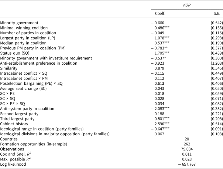
Note: Conditional logit with formation opportunities as observations and potential coalitions in choice set. *p < 0.1; **p < 0.05; ***p < 0.01.
Our model performs similarly to or slightly better than those of Martin and Stevenson (Reference Martin and Stevenson2001, Reference Martin and Stevenson2010), as shown in Appendix Table B1, through the inclusion of six new variables. We use a common government experience indicator in place of a familiarity score; our anti-system party indicator, as defined by Abedi (Reference Abedi2004), replaces the anti-establishment index based on CMP data (Volkens et al., Reference Volkens, Lehmann, Mathhieß, Merz, Regel and Werner2015), because the original variable does not account for how a party's anti-establishment standing is perceived by other parties; and we introduce two new indicators capturing whether a potential coalition contains the second or the third largest party in parliament, as we expect that the coalition inclusion chances of the third largest party, the “kingmaker,” trump those of the second largest party.Footnote 11
Finally, we replace the two log RILE measures of ideological distance in the government and the opposition with two based on party family. For this, we take cues from the results of work done by König et al. (Reference König, Marbach and Osnabrügge2013) whose implications guide us in ordering party families along a latent left-right dimension based on their log RILE scores and assigning integer values increasing by one moving from left to right.Footnote 12 In this way, we lose variation in parties’ ideological positions but we gain a large number of party-election observations.Footnote 13 Moreover, a sequence based on party families still conveys the most important ideological information within each formation opportunity in our conditional logit set-up—who is adjacent to whom—and model performance is nearly identical.Footnote 14, Footnote 15 At the coalition level, we measure distance simply as the absolute distance between the two most extreme parties of a potential coalition. The data stem from ParlGov (Döring and Manow, Reference Döring and Manow2016) and the CMP (Volkens et al., Reference Volkens, Lehmann, Mathhieß, Merz, Regel and Werner2015); for parties in the agrarian party family and for special issue parties, we looked into their international party group affiliation and/or which parliamentary party group they belong to in the European Parliament to approximate their ideological position.
Because the purpose here is not to replicate but to build on previous research to select the best specification for predicting coalition formation, we especially care about out-of-sample prediction. The results suggest that our new variables indeed matter for cabinet formation. Anti-establishment parties fare worse in entering a coalition, while the more frequently a large set of parties within a potential cabinet has recently governed together, the more likely these parties are to eventually form a government. Additionally, being the third largest party in parliament is significantly associated with government formation lending some credibility to the common “kingmaker” analogies. Our party-family based ideology indicator performs roughly as well as the original one based on log RILE scores but with the advantage of a much lower loss of observations in step 3 below.
The Cox and Snell R 2 values reported in Table 2 provide some indication regarding the in-sample predictive performance of our model. The maximum possible value depends on the model's functional form and is reported in the table as well. The R 2 value of our model shows that with our additional regressors we explain only roughly 40 percent of the variance that a perfectly predictive conditional logit would have for the data at hand. Yet, our model slightly outperforms the current state-of-the-art specifications (see online Appendix Table B1).
What matters most for our purposes, however, is to predict correctly the formation of governments beyond the data we used to estimate the coefficients. Table 3 displays the confusion matrix for out-of-sample point predictions for the 62 randomly selected formation opportunities which we set aside as a testing set. For each formation opportunity, we predict that the potential government with the highest predicted probability will form. Hence, barring ties, we should obtain exactly 62 positive predictions. The rows of Table 3 depict our predictions, while the columns report potential governments that actually did or did not form. Thus, the downward diagonal of the matrix contains the correct predictions and the upward diagonal reports the false negatives and false positives.
Table 3. Coalition-level confusion matrix excluding majority situations

Note: Based on our model reported in Table 2 estimated on a training dataset excluding single-party majority situations and predictions tested out-of-sample. Column percentages in parentheses. Precision = TP/(TP + FP); Recall = TP/P.
The out-of-sample predictive performance mirrors the modest in-sample performance of our model. Although we only predict about 48 percent of coalition governments correctly, our model still outperforms the competitor models that at best predict 45 percent (see Table B2 in the online appendix). Prima facie, these findings seem to suggest that our understanding of government formation in non-single-party-majority legislatures remains limited but, as we discuss below, the prediction rate for which parties, in contrast to coalitions, enter government is much higher.
4.2 Step 2: adjusting for majority situations
4.2.1 The KOR_par model
Having identified the most promising predictors of coalition formation on a sample that excluded single-party majority government formation opportunities, we now adjust our model specification to account for such formation opportunities. For this, we introduce interaction terms to capture the conditional effects of our predictors in situations where a single party holds a parliamentary majority and when it does not. As complex models with many predictors usually perform poorly out of sample, we compensate for interactions by reducing the number of predictors. In the following section, we will combine this model with polling data to calculate CIPs. First, however, we must explain the model.
We, unlike much of the coalition formation literature, are interested in the formation of any type of government, including single-party majority cabinets. In order to get the probabilities of inclusion in government right for all parties, we need to know the probability that the majority party will govern alone. We therefore fit an additional model to a dataset that still matches the coverage of Martin and Stevenson (Reference Martin and Stevenson2010)—we will expand the sample in the next step—but includes formation opportunities in single-party majority situations. As most of our indicators are expected to behave differently under single-party majority and non-majority situations, we introduce interaction effects to account for the predictors’ possible diverging effects in these situations. Our model in Table 4 includes the key variables from our model in Table 2, interacted with “no-majority situations”, the abreviation for no-single-party-majority situations. The dummy variable for no-majority situations, of course, cannot enter the model outside of an interaction because it does not vary within choice sets. As parsimonious models are less likely to fit noise and predict best out of sample, we counter the additional complexity introduced by the interactions by dropping a number of predictors that can safely be regarded as non-confounders on theoretical grounds, offer little predictive value, and are laborious to collect. In order to assess the predictive quality of this model, we again randomly sampled 80 percent of the formation opportunities, now including majority situations, into a training dataset onto which we fit the model and reserved 20 percent as a testing sample. As it contains only a subset of the set of previous predictors we denote this model KOR_parsimonious or KOR_par.
Table 4. General model of government formation (KOR_Par)

Note: KOR Parsimonious (KOR_Par) model. Training data. Conditional logit. *p < 0.1; **p < 0.05; ***p < 0.01.
4.2.2 Predictive validity of the KOR_par model
At the coalition level, the KOR parsimonious model (Table 4) outperforms the others, which also have been estimated on the new data, both in- and out-of-sample (see Table D1 in the online appendix). But those are also the wrong metrics for our current purpose. We care, first and foremost, about accurately predicting which parties will be in government, an important distinction from predicting precisely which governments will form. If, for example, our model predicts a given coalition and the true coalition entails the identical composition plus one small surplus party, this is coded at the coalition level as a prediction failure. At the party level, however, all of the predicted parties would be coded as successes and the extra party not predicted by the model would affect only the false-negative rate. Table E1 in the online appendix shows that false positives at the coalition level more often include most of the actual governing parties than predict a fully false coalition.
Most importantly, party-level prediction metrics suggest strong predictive performance. The bottom two rows of Figure 2 present the party-level predictive performance of our KOR (Table 2) and KOR_par (Table 4) models, respectively, both in- and out-of-sample. For comparison, we also include the naïve model and Martin and Stevenson models from 2001 and 2010 from Table B1 in the onlineappendix.

Figure 2 shows that the ROC curve for our parsimonious (KOR_par) model run on the data including the single-party-majority formation opportunities captures 89 percent of the true-positive and false-positive area. Thus, for unknown cases, this model detects the true government participation of actual governing parties 89 percent of the time. While the KOR model performs even slightly better, the other models do not predict outcomes as accurately. We choose the KOR_par model over the KOR model as the basis for predicting CIPs because of its greater parsimony and explicit modeling of the theoretical expectation that key covariates have different effects in majority and non-majority situations.
4.3 Step 3: calculating dynamic CIPs using polls
In the previous two steps, we have identified the most promising indicators by comparing our models to the state-of-the-art (step 1) and by adjusting the resulting model to data including both non-majority and single-party majority situations through the inclusion of interaction effects (step 2). Now that we have settled on a single model—Table 4 (KOR_par)—using data that allowed comparison with previous models, we expand our sample to all available government formation opportunities for which we have both coalition formation and polling data. Concretely, this means adding more recent time periods (up to 2018) and more countries (from Central and Eastern Europe). The additional observations, of course, change the coefficients somewhat, as shown in Table E2 in the online appendix.Footnote 16, Footnote 17
We are now able to calculate the CIPs. By plugging values from polls and other covariates into our KOR_Par coalition formation model, we can predict the probability of all possible coalitions. Note, however, that polls do not enter directly into the KOR_par model, rather they inform several other variables such as the Largest Party, Second Largest Party or Third Largest Party or a Minority Government or a No-Single-Party-Majority Situation. At each formation opportunity, we can then sum up the predicted probabilities over all potential governments k of which party q is part (k = j) in order to calculate the probability of party q being included in government. More specifically, in its simplest form for any given formation opportunity,

where α is a vector of coefficients and x k a vector of predictor variables associated with potential government k. In essence, the CIP of party q is the sum of the probabilities of all governments that include party q. CIPs, of course, can be tailored to match many different bargaining settings. If a researcher, for example, wanted to estimate the bargaining leverage (exit threat) of a junior coalition member on the lead party in a coalition, it is possible to estimate the sum of the probabilities of all possible coalitions that include the junior party and exclude the current lead party. We will make CIP estimates of all such combinations available.
Our polling data include an impressive number of political polls but they are not without gaps and the frequency of polls in different time periods can vary considerably. Both to smooth out noise and to produce coalition inclusion probabilities at regular intervals, we average our polling data by party within months.Footnote 18 Each monthly set of party polling averages is then treated as if it were an election: party poll shares are treated as vote shares which in proportional representation systems approximate seat shares. What matters here is not how well polls predict sometimes distant elections but that politicians interpret them as likely outcomes if an election were to occur at that time. Given that our poll averaging is monthly, our CIP estimates are also monthly.
The result of this exercise is a set of monthly coalition inclusion probabilities for nearly every party in 21 democracies for all years with polling data since 1970. Not only do we estimate the monthly probability of each party entering government but also, for most parties, their probabilities of entering a government that excludes certain other parties. No previous work known to us has (a) as explicitly theorized a dynamic role for coalition leverage and coalition prospects in policy-making and (b) estimated party-level coalition leverage dynamically between elections.Footnote 19 As politics and policy-making do not stop between elections, there is almost no other measure of party-level policy influence available to researchers that can be used to predict policy change between elections. The only other alternative is polling data which, as we have discussed, neglects party characteristics and the coalition inclusion calculus.
4.4 Measure validity
Before we demonstrate the use of our CIP measure in specific applications, it is important to validate it as well as possible. Direct cross-validation is not possible, given that there are no other dynamic measures of credible exit threats, coalition leverage or coalition prospects. However, face validity checks and a test of predictive validity are possible. In the online appendix, we show (1) that the distribution of CIPs for the parties in three distinctly different party systems (Spain, Sweden and Germany) conform to expectations (Section F.1); (2) that CIP values change over time to reflect the different coalition opportunities afforded by small changes in polling over the life of a government (Section F.2); and, for predictive validity, (3) that CIP actually predicts government inclusion (Section F.3).
5. Applications
Are CIPs actually useful for predicting policy? To demonstrate the utility of our CIP measure, we provide two brief applications examining government spending and the stringency of environmental policy as a function of certain parties’ bargaining leverage. We calculate the yearly mean of parties’ monthly CIPs to match the annual frequency of the two dependent variables.
5.1 Government spending
Our first application addresses one of the most central functions in a legislature, that is, deciding on government spending. This spending includes delivering public goods and services or providing social protection and is measured as a percentage of GDP.Footnote 20 Whether to spend more or less has been a perennial dimension of political contention in many democracies over time. We model the year-on-year change in government spending as a function of the previous year's GDP growth, the minority status of the government, the time to the next regular election (in years), the number of cabinet parties as well as the ideological range in the cabinet. As discussed above, we are pitting our CIP estimates against polls, as yearly means for both, and seat shares, which only change at elections. We focus on the prime minister's party (PM) and the party holding the finance ministry (FIN). We expect that with greater leverage, that is, CIPs, government parties, especially the PM and the FIN parties, can stave off demands from other government or opposition parties for greater spending and can keep a tighter hold on the budget.
Table 5 reports results from linear models with country and time period fixed-effects and standard errors clustered by country.Footnote 21 The first two models show null findings for the PM and FIN parties’ polling support. Similar null findings are shown in the third and fourth models using PM and FIN parties’ seat shares. Not only are their coefficients statistically insignificant, but they are nearly zero. In the fifth and sixth models, however, we include the CIPs of the PM and the FIN parties, respectively. As expected, governments tend to spend less compared to the year before when the party holding the finance portfolio sees an increase in its CIP. When the FIN party's CIP moves from 0 to 1, we would expect a drop in government spending of approximately 1.6 percentage points compared to the year prior. Having a greater probability of inclusion in an alternative government provides the FIN party with greater bargaining leverage over other parties making demands—be they in opposition or coalition partners. For the PM party, the effect has a similarly large coefficient but fails, however, to reach conventional levels of significance. Robustness tests in the appendix show consistent effects of the FIN party when accounting for different measures of the party's ideological position and attitude toward Keynesian demand management (see Table G2 in the online Appendix). Next, we turn to an example exploring how CIPs affect government policy legislation.
Table 5. Coalition inclusion probabilities and government spending

Note: Observations differ because we include cabinets wit non-partisan PMs. OLS with country and five-year period fixed-effects. Robust standard errors in parentheses. *p < 0.1; **p < 0.05; ***p < 0.01.
5.2 Environmental policy stringency
In our final example, we highlight the superiority of CIP over polls and seat shares by modeling a legislative outcome: environmental policy. More specifically, we use environmental policy stringency, a composite measure developed by the Organizaton for Economic Cooperation and Development (OECD) with coverage from the 1990s to 2012, as a dependent variable. This indicator focuses primarily on air and climate policies by covering policies related to environmentally relevant taxes, renewable energy and energy efficiency support, performance standards and information on deposit and refund schemes. It ranges as a continuous measure from 0 to 6, with 6 indicating the most stringent policies (Botta and Kozluk, Reference Botta and Kozluk2014).Footnote 22 As this indicator is measured annually, we aggregate polls, seat shares and the CIP of parties belonging to the Ecological/Green Party family to the same frequency by calculating means.
Table 6 presents estimates from linear models with country and period fixed-effects. A set of control variables captures economic feasibility and environmental necessity for action—that is, GDP growth and total greenhouse gas emission per capita—while political controls account for political feasibility, preference for reform and public opinion. We control for cabinet status, the ratification of the Kyoto Protocol, the preference for environmental protection measured by item p501 Environmental Protection: Positive of the Manifesto Project (Volkens et al., Reference Volkens, Lehmann, Mathhieß, Merz, Regel and Werner2015) and for the share of the population worried about the environment. We measure the cabinet's level of mean environmental protection, that is, the mean of item p501 across all governing parties. Public opinion is measured by the weighted share of respondents per country and year answering strongly agree or agree on the item worry about future environment in three waves (1993, 2000, 2010) of the International Social Survey Programme (ISSP). Data points in between have been linearly interpolated.Footnote 23 Finally, we include a dummy-variable for Green Party government participation.
Table 6. Green parties’ influence on environmental policy stringency

Note: OLS with country and five-year period fixed-effects. Robust standard errors in parentheses. *p < 0.1; **p < 0.05; ***p < 0.01.
Central to this model is our CIP measure that captures the probability of each country's green party being included in a new government, were elections to be held. We compare its predictive performance against two non-strategic proxies for policy-influence, polls and, less dynamically, seat shares. In all models, whether included separately or in combination with polls and/or seat share or public opinion, our CIP indicator predicts environmental policy stringency. The more that green parties become necessary for prospective coalition formation, the greater the current government's green policy output. These results could suggest that prime minister parties appeal to or try to subvert green parties by tightening environmental policy once they become a viable coalition partner or threat. Even when green parties are in opposition, the PM party has an incentive to court them through demonstrating policy compatibility (strategic positioning).Footnote 24, Footnote 25 In contrast, the coefficients on the variables for green party polls, seat shares and public opinion—none of which capture the strategic arithmetic of coalition formation—actually host signs suggesting that they reduce environmental stringency and none reaches statistical significance.
6. Conclusion
Political parties are strategic, yet no empirically validated measure exists to capture parties’ incentives to trade-off policy against another top priority, government inclusion. Cabinet parties able to credibly threaten to abandon the current government for an alternative, especially if it would exclude a cabinet policy rival, have high credibility and bargaining leverage as shown in our applications. Likewise, opposition parties that are important to the formation of future coalitions have policy leverage as well. By estimating and distributing a measure that captures a quantity central to parties’ strategic calculations and by doing so both broadly and dynamically—for all relevant parties in 21 countries over multiple decades at a monthly frequency—we hope that the measures that we provide can enable scholars to investigate a broad swath of new research into a large variety of political and policy-making behavior.
Supplementary material
The supplementary material for this article can be found at https://doi.org/10.1017/psrm.2021.75.
To obtain replication material for this article, please visit https://doi.org/10.7910/DVN/GUKPZO
Acknowledgments
We kindly thank Jon Fiva, Evenlyn Hübscher, Rene Lindstädt, Lanny Martin, Anthony McGann, Thomas Sattler and Georg Vanberg for helpful comments. We further thank Lanny Martin, Will Jennings, Christopher Wlezien and Christopher Wratil for sharing data with us. Mark Kayser and Jochen Rehmert gratefully acknowledge support from the German Federal Ministry for Education and Research (BMBF), grant number 01UF1508. Our coalition inclusion data will be made available online at coalition-leverage.org and updated periodically.


 Open access