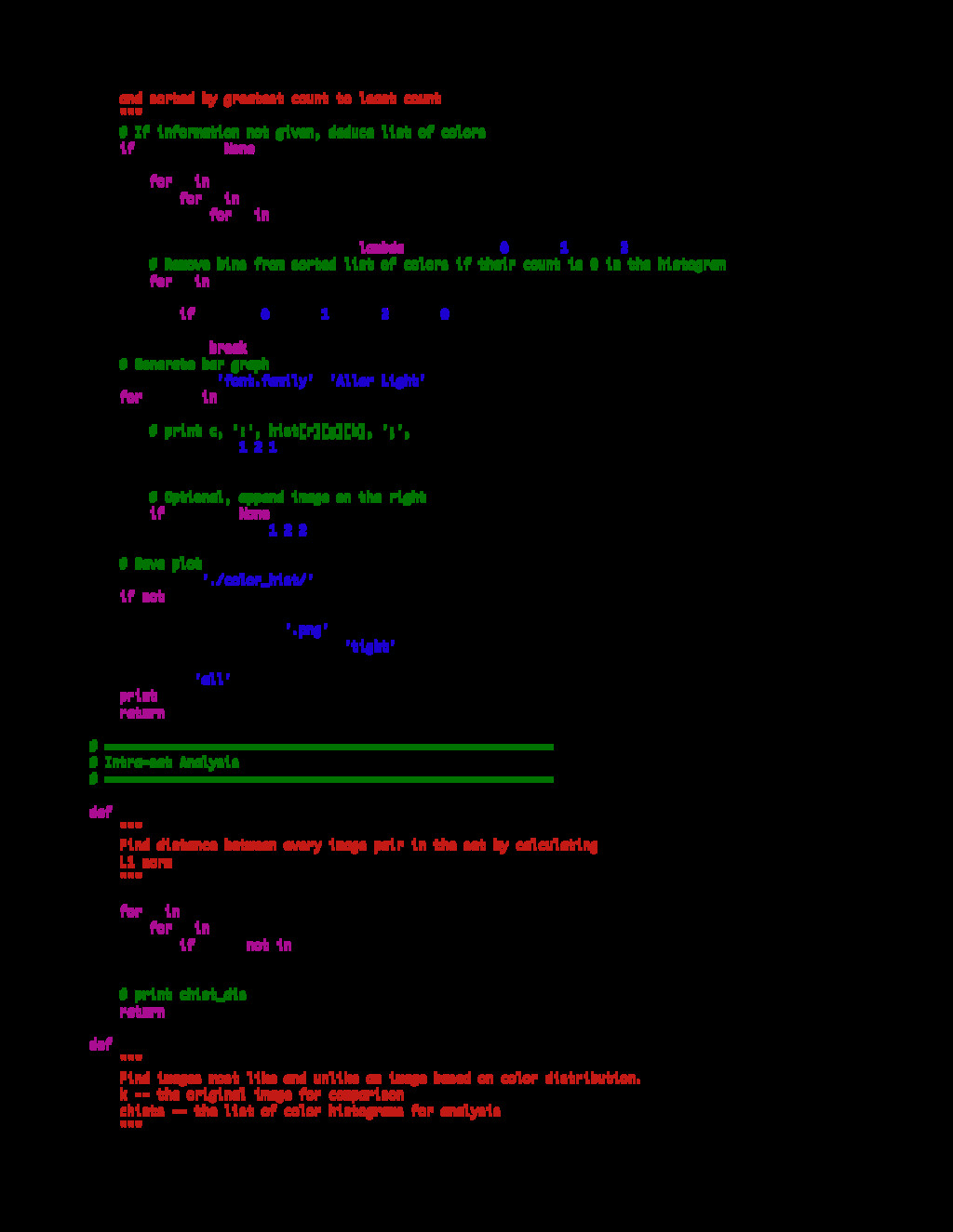
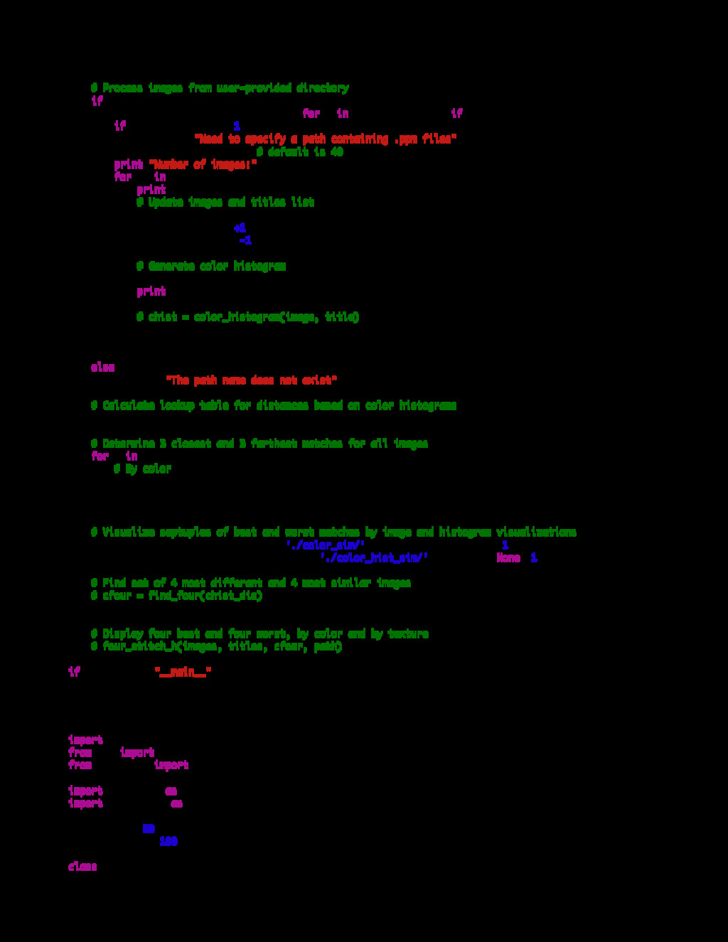
= [] for i in xrange(0, NUM_IM): if k > i: # because tuples always begin with lower index results[i] = chist_dis[(i,k)] else: results[i] = chist_dis[(k,i)] # Ordered list of tuples (dist, idx) from most to least similar # -- first value will be the original image with diff of 0 results = sorted([(v, k) for (k, v) in results.items()]) # print 'results for image', k, results seven = results[:4] seven.extend(results[-3:]) # print 'last seven for image', k, seven distances, indices = zip(*seven) # print 'distances:',distances # print 'indices:',indices return indices, distances def find_four(chist_dis): results = {} # ensure that a<b, b<c and c<d as order does not matter for a in xrange(NUM_IM): for b in xrange(a+1,NUM_IM): for c in xrange(b+1,NUM_IM): for d in xrange(c+1,NUM_IM): results[(a,b,c,d)] = \ chist_dis[(a,b)] + chist_dis[(a,c)] + \ chist_dis[(a,d)] + chist_dis[(b,c)] + \ chist_dis[(b,d)] + chist_dis[(c,d)] results = sorted([(v, k) for (k, v) in results.items()]) best = results[0] worst = results[-1] indices = list(best[1]) indices.extend(list(worst[1])) # print "results: ", len(results), #results # print "best, worst", best, worst return indices # ============================================================ # Intra-Set Visualization # ============================================================ def septuple_stitch_h(images, titles, dir_name, cresults, cdistances, cvt): plt.rcParams['font.family']='Aller Light' gs1 = gridspec.GridSpec(1,7) gs1.update(wspace=0.05, hspace=0.05) # set the spacing between axes. for k in xrange(0, NUM_IM*7, 7): for i in xrange(7): idx = cresults[k+i] ax = plt.subplot(gs1[i]) plt.axis('on') if cvt is 0: plt.imshow(images[idx], cmap="Greys_r") elif cvt is -1: plt.imshow(images[idx], cmap="binary") else: plt.imshow(cv2.cvtColor(images[idx], cv2.COLOR_BGR2RGB)) # row, col plt.xticks([]),plt.yticks([]) if cdistances: if i == 0:
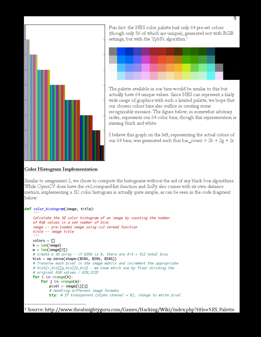
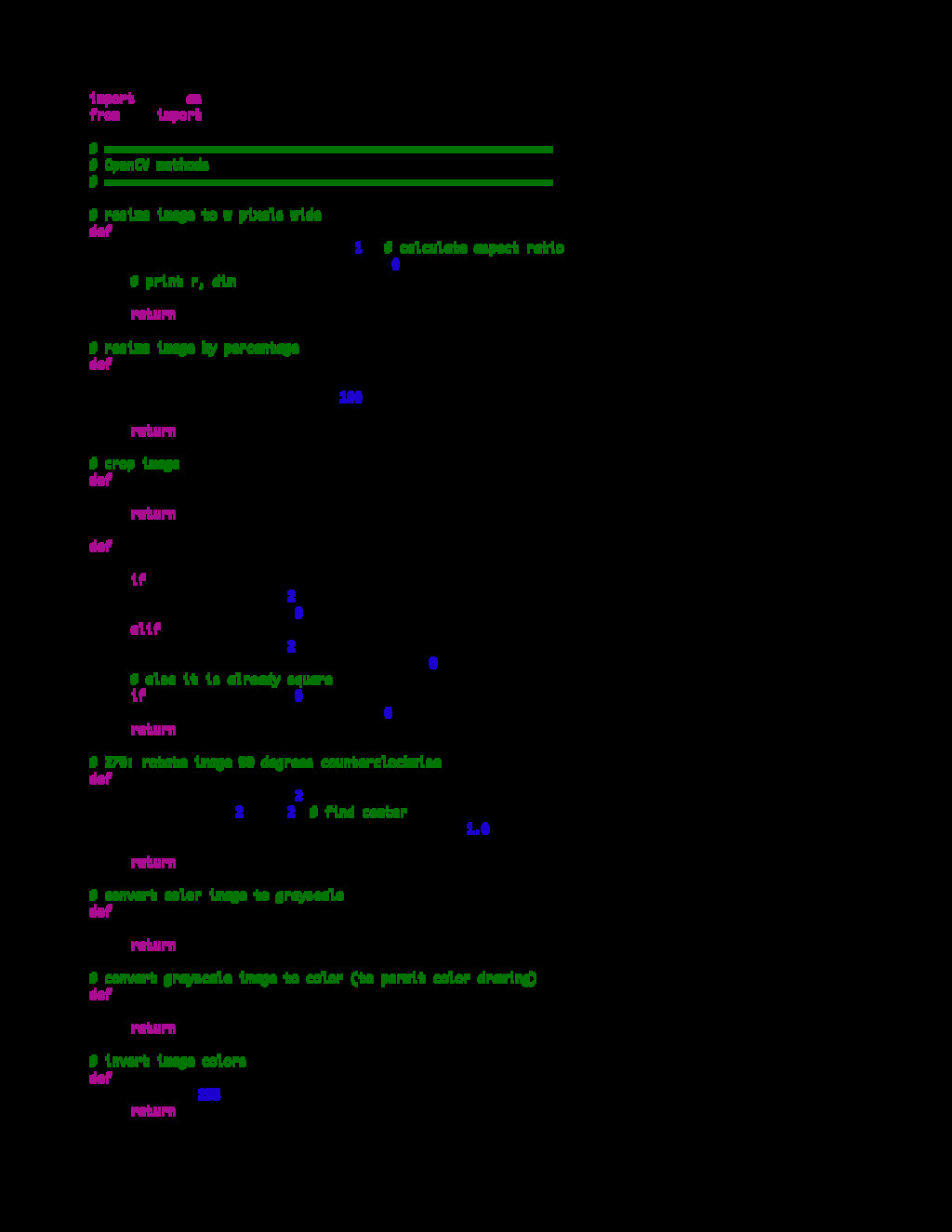
![10 if pixel[3] == 0: pixel[0] = 255](https://files.speakerdeck.com/presentations/9fae67cf6b444acca3dee4ee151c0f4c/slide_9.jpg)
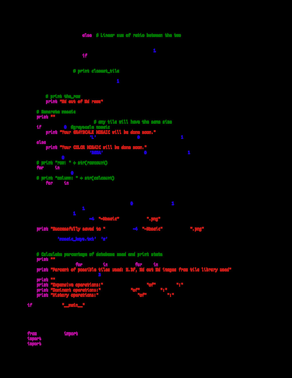
![20 closest_tile = history[str(histogram)] # This constant-time lookup](https://files.speakerdeck.com/presentations/9fae67cf6b444acca3dee4ee151c0f4c/slide_19.jpg)
![22 if dom in dominants: closest_tile = random.choice(dominants[dom])](https://files.speakerdeck.com/presentations/9fae67cf6b444acca3dee4ee151c0f4c/slide_21.jpg)
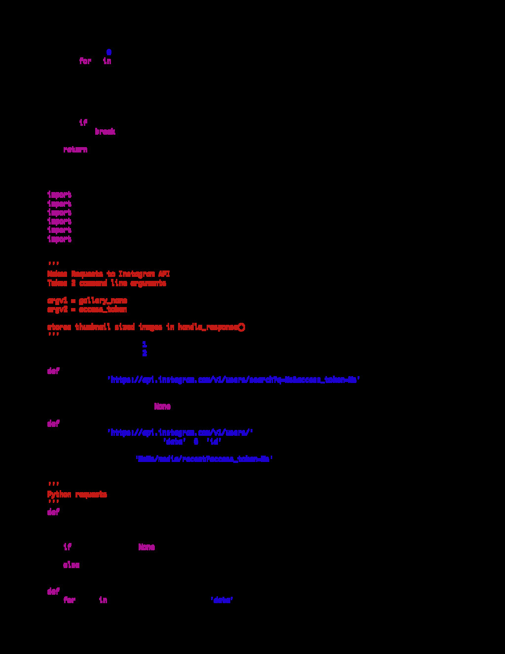
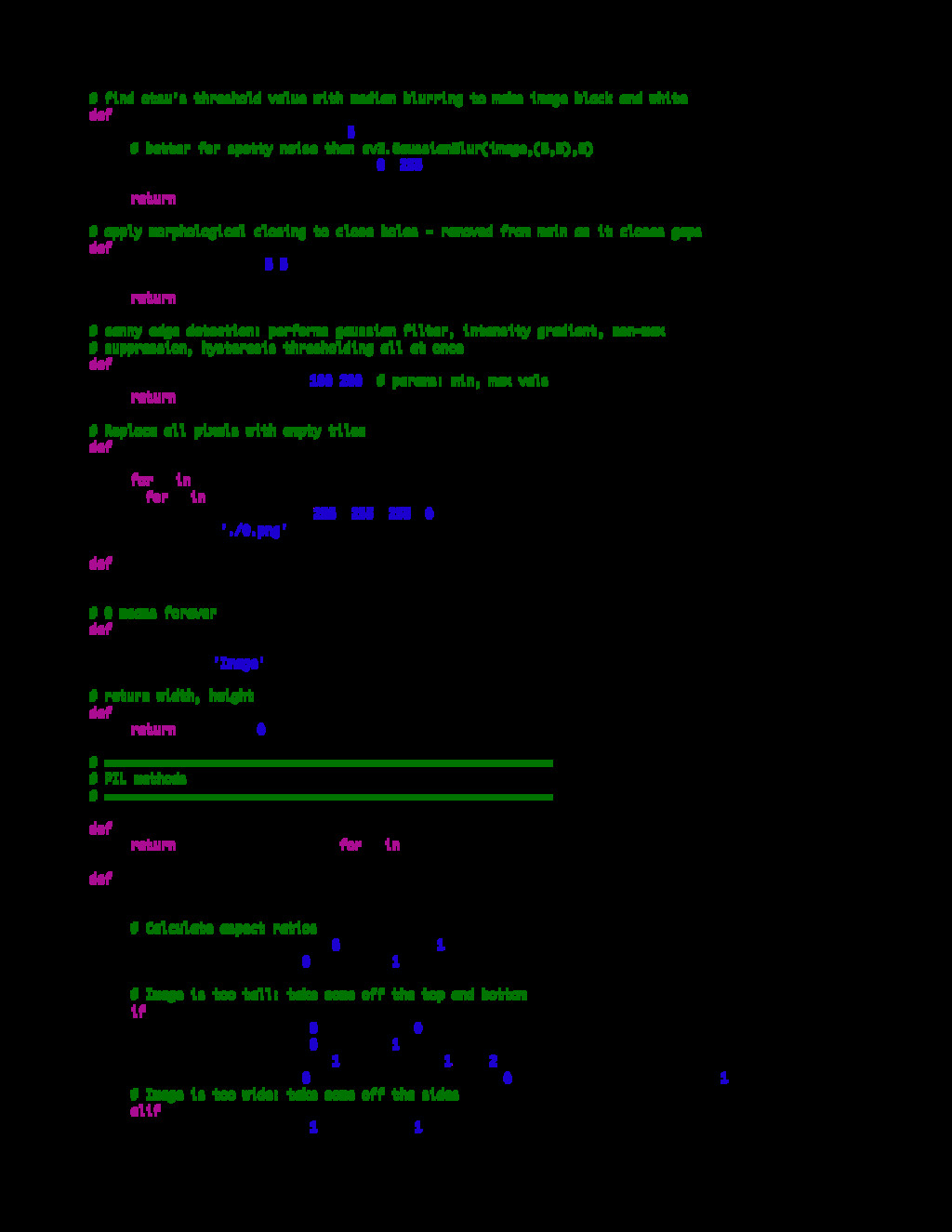
![47 content = parsed_request['data'][item] image_key = content['created_time'] imagePath](https://files.speakerdeck.com/presentations/9fae67cf6b444acca3dee4ee151c0f4c/slide_46.jpg)
![49 else: dominants[color] = [tile] # Save tiles](https://files.speakerdeck.com/presentations/9fae67cf6b444acca3dee4ee151c0f4c/slide_48.jpg)
![53 crop_size = (target[0]/scale_factor, original[1]) side_cut_line = (original[0]](https://files.speakerdeck.com/presentations/9fae67cf6b444acca3dee4ee151c0f4c/slide_52.jpg)
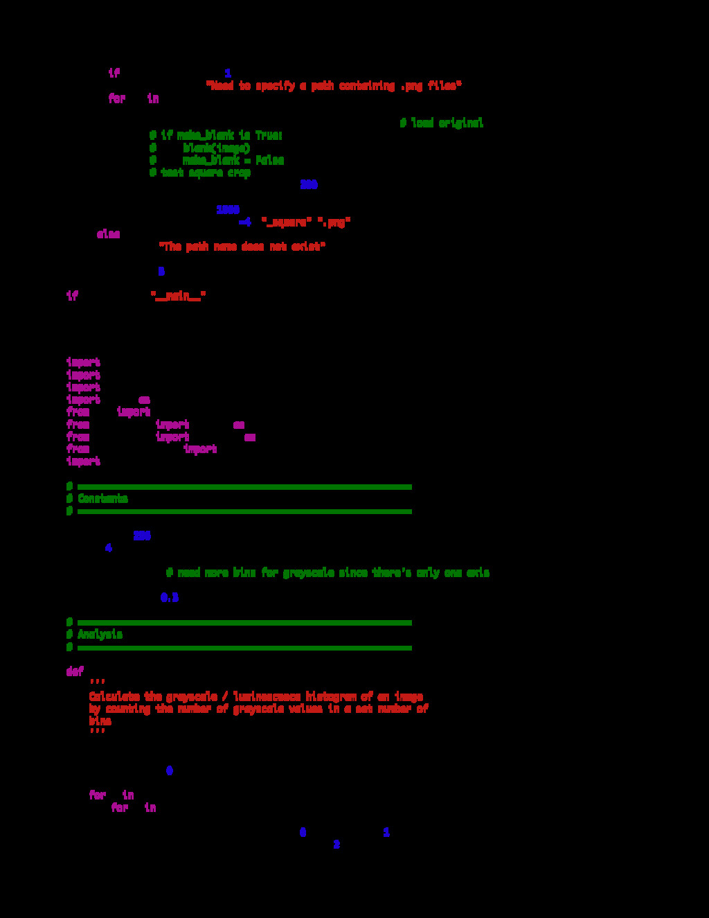
![55 gray = gray/3 g_bin = gray/gBIN_SIZE hist[g_bin]](https://files.speakerdeck.com/presentations/9fae67cf6b444acca3dee4ee151c0f4c/slide_54.jpg)
![56 diff += abs(h1[g]-h2[g]) total += h1[g]+h2[g] l1_norm](https://files.speakerdeck.com/presentations/9fae67cf6b444acca3dee4ee151c0f4c/slide_55.jpg)
![58 results = {} indices = [] distances](https://files.speakerdeck.com/presentations/9fae67cf6b444acca3dee4ee151c0f4c/slide_57.jpg)
![59 plt.xlabel('similarity:') else: sim = 1 - round(cdistances[k+i],](https://files.speakerdeck.com/presentations/9fae67cf6b444acca3dee4ee151c0f4c/slide_58.jpg)