

Abstract
We assess the utility of seasonal forecasts for the energy industry by showing how recently-established predictability of the North Atlantic Oscillation (NAO) in winter allows predictability of near-surface wind speed and air temperature and therefore energy supply and demand respectively. Our seasonal prediction system (GloSea5) successfully reproduces the influence of the NAO on European climate, leading to skilful forecasts of wind speed and wind power and hence wind driven energy supply. Temperature is skilfully forecast using the observed temperature-NAO relationship and the NAO forecast. Using the correlation between forecast NAO and observed GB electricity demand, we demonstrate that skilful predictions of winter demand are also achievable on seasonal timescales well in advance of the season. Finally, good reliability of probabilistic forecasts of above/below-average wind speed and temperature is also demonstrated.
Export citation and abstract BibTeX RIS

Original content from this work may be used under the terms of the Creative Commons Attribution 3.0 licence. Any further distribution of this work must maintain attribution to the author(s) and the title of the work, journal citation and DOI.
1. Introduction
For sectors of industry and the economy influenced by inter-annual climate variability, good seasonal predictability of climate potentially offers considerable socio-economical benefits (e.g. Palin et al 2016, Emanuel et al 2012, Cantelaube and Terres 2005, Challinor et al 2005, Morse et al 2005, Katz and Ehrendorfer 2005, Svensson et al 2015, Palmer 2002, Karpechko et al 2015). Reliable forewarning of cold, calm winters for example could help decision makers in the energy industry plan resources effectively to minimise the risk of power shortages and price shocks from mismatches in supply and demand. Many studies have recognised the utility of a skilful seasonal forecast for the energy industry (e.g. Troccoli 2010, Brayshaw et al 2011, Buontempo et al 2010), but although Soares and Dessai (2015) found the energy industry was relatively advanced in the use of seasonal forecast information compared to other sectors, there are few published studies on actual use (De Felice et al 2015 is a rare example).
For some aspects of the climate system, for example sea surface temperatures and tropical circulation, predictability at seasonal lead times has been steadily increasing in recent years as a result of improved climate models, assimilation of initial conditions and ensemble production techniques (e.g. MacLachlan et al 2015, Kirtman et al 2014, Kim et al 2012, Arribas et al 2011, Balmaseda et al 2010, Doblas-Reyes et al 2009). For mid-latitude regions though, such as Northern Europe, good predictability of fields useful for climate services, for example of near-surface wind speed and temperature has, until recently, remained elusive (Smith et al 2012). However, with the latest forecast systems, significant extratropical winter prediction skill is, finally, now a reality (Scaife et al 2014, Athanasiadis et al 2015, Siegert et al 2015, Kang et al 2014, Riddle et al 2013). Scaife et al for example, report a correlation of 0.6 (statistically significant at 1% level) between seasonal mean values of model simulated and observed surface NAO, for the 20 years from 1993 to 2012. The NAO is defined here as the difference in sea level pressure during winter between two regions of predominantly high and low pressure (the Azores and Iceland respectively, (Hurrell 1995, Johansson 2007) and its improved predictability has particular relevance for the climate variables of interest to the energy industry. Aspects of this relevance are discussed in section 3 of this article, after a brief description of the seasonal forecast system in section 2.
In section 4 we consider the reliability of the forecast system. It is essential to establish the extent to which the probabilities of forecast events (like a warmer-than-average winter) can be relied upon for decision-making, and that the forecast system isn't overconfident (Weisheimer and Palmer 2014) or under-confident (Eade et al 2014, Kumar et al 2014). However, unlike correlation skill, the reliability of the forecast system can be improved through calibration, once the behaviour of the raw model forecasts (which we show here) is known.
Finally in section 5, we assess the degree to which GloSea5 can be used to predict inter-annual fluctuations in energy demand by comparing seasonal climate predictions with observed statistics provided by the UK energy industry.
2. Data and methods
We use data from the Met Office GloSea5 (Global Seasonal forecast system 5) simulations comprising 20 years of December to February (hereafter DJF), hindcasts initialised between October 25th and November 9th prior to each winter. Twenty-four simulations in total were available for each year using a combination of lagged initialisation dates and stochastic physics as described in MacLachlan et al (2015). These forecasts were produced with the coupled Met Office HadGEM3 climate model with atmosphere, land, ocean and sea-ice components provided by the Met Office Unified Model and JULES (GA3.0/GL3.0 configuration, Walters et al 2011), NEMO (GO3.0 configuration, Madec 2008) and CICE (GSI3.0 configuration, Hunke et al 2004) models respectively. Resolutions of the components are given in table 1 and are relatively high with 0.25 ° ocean resolution and less than 1 ° in the atmosphere. We refer readers to the references above for more complete details of the models and model configurations used.
Table 1. GloSea5 resolution
| Horizontal | Vertical | |
|---|---|---|
| Atmosphere | N216 (approx. 50 km at 50 °N) | 85 levels with highest at 85 km |
| Ocean | ORCA0.25 (0.25° lat, long, approx. 27 km at equator) | 75 levels |
Throughout this article we use ERA Interim (Dee et al 2011) reanalyses to represent historical observations.
3. Relevance of the NAO to European wind and temperature
Before we quantify the influence of the NAO on near-surface wind and temperature, it is worth considering the skill of the sea level pressure forecasts from which the NAO is derived. To do this, figure 1 shows a map of the correlation between observed and predicted seasonal means of sea level pressure for winter (DJF). Point correlation for this season exceeds 0.4 (statistically significant at 10% level, using a t-test) for the individual regions of climatological low and high pressure over Iceland and the Azores respectively which form the NAO dipole. Spatially, the skill varies little, suggesting that the winter NAO skill reported in Scaife at al is insensitive to the specific NAO definition (e.g. by using empirical orthogonal function (EOF) analysis to define the NAO rather than using predefined locations of the NAO centres of action).

Figure 1 Correlation between GloSea5 ensemble mean and ERA Interim sea level pressure for DJF compiled from 20 years of simulation. Mask (white areas) applied to correlations not significantly greater than zero at 10% level.
Download figure:
Standard image High-resolution imageThe NAO is a well known driver of inter-annual climate variability in Northern Europe for sound physical reasons (e.g. Luterbacher et al 2004, Trigo et al 2002, Pozo-Vázquez et al 2001, Hurrell 1996) and can alter the frequency of extreme events (Scaife et al 2008, Thompson et al 2002). The meridional pressure gradient it describes largely determines the strength of the westerly wind in north-western Europe by geostrophic balance. Observed winters in this region are therefore usually windy and mild when the NAO is anomalously positive (Folland et al 2012, Neill et al 2014) but calm and cold when negative (e.g. Jung et al 2011, Scaife and Knight 2008, Fereday et al 2012, Maidens et al 2013). The opposite relations hold in south-western Europe. Replication of these observed teleconnections is thus a requirement of seasonal prediction systems in order to achieve robust predictability of near-surface wind speed and temperature. These are shown in figure 2. Regions coloured red are windier than usual during anomalously positive NAO winters and blue where calmer than usual. The GloSea5 seasonal forecast system replicates the observed patterns remarkably well, reproducing the strong latitude dependence of the NAO on near surface wind speed. There is also a large scale relationship between the observed NAO and temperature across Europe (figure 2, right column) with positive NAO winters being the warmest. GloSea5 replicates this reasonably well (right column, middle row) but its ensemble mean (bottom right) shows a weaker correlation which explains the weaker level of skill in temperature forecasts for this region (Scaife et al 2014).
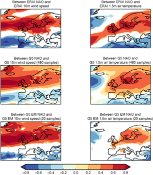
Figure 2 Correlations between NAO on winter near-surface wind speed (left column) and temperature (right column). Observed (ERA Interim) relationships are shown in the top row. Middle row shows ensemble member relationships in hindcasts. Bottom row shows ensemble mean relationships in hindcasts. Mask (white areas) applied to correlations not significant at 10% level.
Download figure:
Standard image High-resolution image4. Wind speed, power and temperature seasonal forecast skill and reliability
Figure 3 shows some diagnostics of relevance to the energy industry. The first is a time-series of near-surface wind speed for the UK (10 °W, 50 °N to 3 °E, 60 °N) with a correlation of 0.64 between the GloSea5 ensemble mean and ERA Interim. For each data set, the wind speeds are normalised by subtracting the climatological winter mean and dividing by the standard deviation. This is necessary because the inter-annual variability of the ensemble mean is considerably smaller than that observed (2% of mean absolute wind speed values compared to 8%).
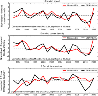
Figure 3 Time series of GloSea5 hindcast (red) and observed (ERA Interim, black) DJF mean near-surface wind speed, power density (0.5ρU3 where ρ is the air density and U is the daily mean wind speed) and temperature, averaged over the UK.
Download figure:
Standard image High-resolution imageThe second series is for wind power density, produced using power density = ½(ρU3) where U is the wind speed at 10 m (in m s−1), following the approach of Manwell et al (2010) in which wind power is primarily a function of the volume throughput of air driving the blades of a turbine. ρ is the air density, computed here using the ideal gas law (ρ = P/RT), where P, T and R are the pressure, temperature and specific gas constant for dry air (287.058 J kg−1 K−1) respectively. For reasons of data availability, we use pressure at mean sea level and temperature at 2 m. Seasonal means of power density were produced for each gridpoint by averaging over power densities computed using the daily-mean output from the GloSea5 hindcasts and 6-hourly means from the ERA Interim verifying reanalysis. Data at finer temporal resolution (which was not available) would have been preferred for this analysis, since the mean of U3 is only equal to the cube of daily mean U in the absence of sub-daily variability. The correlation with power density is slightly smaller (0.58) but still potentially useful and highly significant. The observed extreme winters of 2009, 2010 and 2011 are also clearly predicted by the hindcasts suggesting GloSea5 is of benefit in planning for extreme worst case events. Normalised values are again presented in figure 3, given the smaller standard deviation of GloSea5 compared to ERAI (7% and 20% of mean absolute values respectively).
Further analysis (not shown) has found a strong relationship between winter mean wind speeds at 10m and those at 975 hPa, 950 hPa and 925 hPa in ERAI (correlations of 0.97 ± 0.01 for all 3 levels). Consequently, the results shown here are also likely to be valid for hub height wind speeds (80 m to 130 m above the surface).
The third time series is for temperature, with a correlation of 0.27. For temperature however, better forecasts can be made (0.44 correlation) by simple linear regression using the NAO itself as the predictor. The stronger real-world influence of the NAO on UK temperature, shown in the top right panel of figure 2, compared to that simulated by the ensemble mean in the model (middle right panel of figure 2) is thought to contribute to this improvement as well as greater real world predictability compared to that of the Glosea5 ensemble mean (Eade, 2014). Sensitivity of the skill to the definition of the UK region, tested by displacing the region by half its northerly and easterly extent as well as its size was found to be small (not shown).
Time series of ensemble means and correlations provide a good guide to certain aspects of the performance of a forecast system. However, seasonal predictions are often issued as the probability of a specific event occurring which requires an alternative assessment method. Model reliability describes how closely the forecast probabilities of an event correspond to observed frequencies of that event in the real world (Wilks 2006). For example, a winter wind speed might be forecast to be above-average with 60% probability. Using the hindcast, we could find all the historical winters when it was forecast to be above-average with 60% probability, and count how many of them were actually observed to be above-average. For a 'reliable' forecast system, this should also be around 60% so that forecast probability matches the observed frequency. This information can be gathered from the hindcast and observational data for a range of forecast-probability categories, and plotted as a reliability diagram (observed frequency against forecast probability). For a perfectly reliable system, the points for each probability bin will lie on the 1:1 line.
However, the system could be overconfident, where the event is observed to occur less frequently than predicted when it is forecast with high probabilities, and more frequently than predicted when it is forecast with low probabilities. This results in a line with a slope shallower than 1 on a reliability diagram. Similarly it can be underconfident, forecasting less extreme probabilities than observed, resulting in a gradient steeper than 1 on the reliability diagram (e.g. figure 4 right). Knowing the behaviour of the forecast system in this way allows the system to be calibrated to produce reliable probabilistic forecasts.

Figure 4 Reliability (top) and sharpness (bottom) diagrams compiled from UK region grid cells (following the WMO (2010) standard procedure, see text) for forecasts of winter above-median near-surface air temperature (left) and wind speed (right). The best-fit lines and their uncertainties are shown in pink. The horizontal and vertical dotted lines mark 'no resolution', i.e. they show the climatological frequency of 0.5 (as we are using above-median forecasts). The solid black 1:1 line marks 'perfect reliability', where observed frequencies match forecast probabilities. The red diagonal dashed line is midway between perfect reliability and no resolution, and marks 'no skill'; points above that line (in the green area) make a positive contribution to the Brier skill score (Wilks 2006).
Download figure:
Standard image High-resolution imageRelated concepts are sharpness and resolution. The sharpness of a forecast system refers to its ability to forecast extreme probabilities, rather than just the climatological average. This is shown in the sharpness diagram in the bottom panel of our reliability diagrams, as a histogram of the forecast probabilities in the hindcast data. Ideally, these histograms should be flat across all probability categories, such that the hindcast has a good sample of data at all probabilities with which to judge the reliability. A system that is not sharp will always produce probabilities at the climatological level, with a strongly-peaked sharpness diagram. The combination of the reliability and sharpness diagrams fully describes the joint distribution of the hindcast and observational data (Wilks 2006).
The forecast resolution refers to the ability of the system to resolve the set of forecast events into groups (probability categories) which have different observed frequencies. The 'no resolution' case, where all forecast probabilities correspond to observational frequencies at the climatological rate, is marked on the reliability diagram as a horizontal line.
Figure 4 shows reliability diagrams for above-average wind speed and temperature, following Wilks (2006) and the WMO (2010) standard procedure including cross-validation. We aggregate the hindcast data from each grid cell in our UK region when calculating the forecast probabilities and quantiles. We primarily focus on above-median events to ensure results are as robust as possible, given the limited number of years available. Reliability diagrams for terciles and outer quintile events are however available in the supplementary information but should be treated with caution because of the smaller sample sizes of the data used in their computation. Nevertheless, an increased probability of above/below average events can point towards a greater risk of associated extremes. In our diagrams, we also include the best-fit lines and their uncertainties, calculated using weighted least squares, taking the uncertainty in the forecast probabilities due to the sampling into account. The uncertainties in the gradient of the fit are given by the 75% confidence limits (following Weisheimer and Palmer, 2014) calculated using two-tailed t-tests.
The results for above-median temperature forecasts show good reliability, with a gradient consistent with unity (0.94 ± 0.16). Following the reliability classification of Weisheimer and Palmer (2014), the temperature forecasts for the UK are in the 'perfect' category (see table 2 for details of the category definitions). However, the model sharpness shows a peak around probabilities of 50%–60%, with fewer high-probability forecasts, resulting in the reliability line being noisier at the upper end.
For wind speeds however, the model is underconfident: the gradient of the best-fit line, 1.51 ± 0.12, is significantly greater than 1. This unusual situation is in accordance with Scaife et al (2014) and Eade et al (2014), who discuss the issues surrounding the under-confidence of seasonal and decadal predictions in the Atlantic in more detail, and which has been considered more generally by Kumar et al (2014). In terms of sharpness, GloSea5 appears to produce most wind speed forecasts with probabilities of between 50% and 60%, and with very few low and high probabilities. The underconfidence and deficient sharpness shows the system would benefit from calibration of raw forecasts.
Figure 5 puts the reliability findings from figure 4 into a wider context by showing a map of the reliability categories across Europe, based on the Weisheimer and Palmer (2014) classification (table 2 here). These are more informative than simply mapping the reliability curve gradient, as they take the uncertainty in the best-fit lines into account. For each grid cell, we calculate reliability-diagram information for the rectangular region defined by ±8 grid cells in longitude and ±8 grid cells in latitude (the size of such a box is shown as an example on the map). The gradient of the reliability line and its uncertainty are used to determine the reliability category for that grid cell.

Figure 5 Maps of reliability category, following Weisheimer and Palmer (2014), for GloSea5 hindcasts of above-median air temperature (left) and wind speed (right). The category definitions are described in table 2. Note that we have added an additional category 6 for underconfident forecasts, which dominate the British Isles area for wind speeds. The black box demonstrates the size of the moving window used to produce reliability estimates at each grid point, comprising 17 × 17 grid cells.
Download figure:
Standard image High-resolution imageTable 2. Reliability category definitions. The definitions for categories 1–5 correspond to those of Weisheimer and Palmer (2014). Category 6 has been added here to account for underconfident forecasts. In this table, R refers to the gradient of the best-fit line to the reliability diagram. The lower and upper bounds of the 75% confidence limits are denoted Rlo and Rhi respectively, and the gradient of the 'no skill' line is denoted Rnoskill.
| Category | Definition |
|---|---|
| 6 'underconfident' | Rlo > 1 |
| 5 'perfect reliability' | Rhi ≥ 1 and Rnoskill ≤ Rlo ≤ 1 |
| 4 'still very useful for decision making' | Rhi < 1 and Rlo ≥ 0.5 |
| 3 'marginally useful' | 0 < Rlo ≤ 0.5 |
| 2 'not useful' | R ≥ 0 and Rhi > 0 and Rlo < 0 |
| 1 'dangerously useless' | R < 0 |
For forecasts of above-median temperature, the British Isles is in a category-5 area, indicating perfect reliability (as seen in figure 4). Much of continental Europe however is in category 3 ('marginally useful'); Scaife et al (2014) showed that the skill in forecasting temperature is also much lower in these regions.
For the wind speed, there is a large region around the British Isles where GloSea5 produces underconfident forecasts (category 6), as suggested in figure 4. This shows that that result was not confined to the particular region we chose, and is in fact a large-scale feature in the GloSea5 system.
Good levels of reliability are maintained for wind speed forecasts in France and the North Sea, in contrast to our results for temperature. Again, this corresponds broadly to the area of higher correlation skill shown in Scaife et al (2014).
Overall, our results show that these seasonal forecasts are reliable enough to be useful for the energy sector.
5. Predictability of energy demand
Temperature is an important driver of Britain's electricity demand. For example, two-thirds of the variability of daily electricity demand is linearly accounted for by daily temperature variability, after socio-economic influences have been removed (Thornton et al 2016). In addition to temperature, the grid operators also use forecasts of wind speed and solar irradiance to improve their day ahead demand forecasts (Taylor and Buizza 2003). Given the strong relationship between the NAO and climate over Britain, and the higher predictability of the NAO compared to individual climate components, especially temperature, we assess the predictability of demand using the NAO directly.
We compare observed winter mean GB total electricity demand, with observed and GloSea5 predicted NAO (figure 6). Prior to comparison, we remove low frequency variability from the daily electricity demand timeseries provided by National Grid, as this is thought to be predominantly driven by socioeconomic changes (for further details see Thornton et al 2016).

Figure 6 Top row: Timeseries (left) and scatter plot (right) of standardised observed winter mean NAO index and GB Electricity demand. Bottom row: as top but with NAO from GloSea5 hindcast.
Download figure:
Standard image High-resolution image
The linear relationship between the observed NAO and electricity demand is strong with a correlation of −0.67, statistically significant at the 1% level (figure 6, top). In winter, temperature and electricity demand are strongly anti-correlated, r = 0.8 (Thornton et al 2016). The strong anti-correlation between the NAO and electricity demand therefore has the expected sign and arises principally from the NAO's influence on temperature as discussed earlier.
From the bottom panels of figure 6, the correlation between the predicted NAO and observed electricity demand is also strong (r = 0.57, significant at 1% level). This result suggests for the first time, that skilful real time seasonal forecasts of the weather dependent component of Britain's winter electricity demand are achievable. A skilful forecast of winter mean electricity demand from the preceeding November offers many potential benefits. For example advance warning of very low temperatures and hence high demand, would allow the grid operator to contract additional supply or pursue demand reduction options. Individual plant operators could also reconsider scheduled maintenance outages.
Discussion and conclusions
Deterministic and probabilistic skill of the Met Office's seasonal forecast system has been assessed for the 20 year period from 1993 to 2012. Statistically significant predictability has been shown to occur for mean sea level pressure for most of western Europe and consistent with the NAO skill reported by Scaife et al (2014).
The forecast ensemble successfully reproduces the observed patterns of the influence of the NAO on near-surface wind speed and temperature. This is essential to ensure that the good predictability of the NAO follows through to that of weather diagnostics in Europe, allowing forecasts useful for industry to be made.
Analysis also suggests that for Europe, real-time seasonal forecasts of near-surface wind speed and temperature for energy supply forecasting are reliable enough to be useful. The system does however have a tendency to be underconfident in the prediction of atmospheric circulation and wind speed while direct temperature forecasts also show weaker skill.
Strong, statistically significant relationships have also been demonstrated between observed UK electricity demand and both the observed and predicted NAO. This suggests that skilful seasonal predictions of winter energy demand are possible. Similar results could be expected for other Northern European countries or other applications with similar sensitivity to the winter NAO (e.g. Karpechko et al 2015, Palin et al 2016, Svensson et al 2015). The skill in forecasting the winter NAO could also be useful for energy management in southern parts of Europe. For example in Spain, wind and hydro power are higher during negative NAO winters compared to positive NAO winters, whilst solar power is lower (Jerez et al 2013).
Acknowledgments
This work was supported by the joint DECC/Defra Met Office Hadley Centre Climate Programme (GA01101). AAS was supported by the joint DECC/Defra Met Office Hadley Centre Climate Programme (GA01101) and the EU SPECS project (GA308378).